Overview

ROTIR reconstructs temperature maps on the surface of stars using optical interferometry data. This page explains the core concepts and the typical workflow.

Concepts

Tessellation. The stellar surface is divided into pixels (quadrilateral patches) using either a HEALPix scheme or a longitude/latitude grid. Each pixel has 4 corner vertices and a center, stored in both Cartesian and spherical coordinates on a unit sphere.

Surface geometry. The unit-sphere tessellation is scaled to the physical stellar shape: a sphere, triaxial ellipsoid, rapid rotator (centrifugally distorted), or Roche-lobe-filling star in a binary. The geometry also determines gravity darkening via the von Zeipel law.

Rotation and projection. For each observing epoch, the star is rotated according to its spin period, inclination, and position angle, then projected onto the observer's sky plane. Pixels facing away from the observer are masked (with a smooth sigmoid transition for gradient-based optimization).

Polygon Fourier transform. Each projected pixel is a quadrilateral. Its Fourier transform contribution at each UV frequency is computed analytically using the polygon FT formula (edge-based sinc integrals). The total complex visibility is the flux-weighted sum over all visible pixels.

Direct imaging. In addition to the polyft matrix, ROTIR provides two fast methods for producing real-space images: rasterization (exact polygon-pixel clipping via Sutherland-Hodgman) and NFFT (Gauss-Legendre quadrature folded into a non-uniform FFT). Both avoid the dense polyft matrix and are useful for visualization, image-plane fitting, and large grids. See Direct imaging methods for details.

Reconstruction. The temperature map is optimized to minimize the chi-squared between model and observed interferometric quantities (V², closure phase, triple amplitude), subject to regularization. ROTIR uses the VMLMB quasi-Newton optimizer with analytical gradients.

Minimal workflow

using ROTIR

# 1. Load multi-epoch OIFITS data
oifitsfiles = ["epoch1.oifits", "epoch2.oifits", "epoch3.oifits"]
data_all = readoifits_multiepochs(oifitsfiles)
data = data_all[1, :]                            # first wavelength bin, all epochs
tepochs = [d.mean_mjd for d in data]
tepochs = tepochs .- tepochs[1]                  # relative MJDs

# 2. Create tessellation
n = 3                                            # HEALPix level (npix = 768)
tessels = tessellation_healpix(n)

# 3. Define stellar parameters
star_params = (
    surface_type    = 2,        # 0=sphere, 1=ellipsoid, 2=rapid rotator, 3=Roche
    rpole           = 1.37,     # polar radius (mas)
    tpole           = 4800.0,   # polar temperature (K)
    ldtype          = 3,        # limb darkening: 1=linear, 2=quadratic, 3=Hestroffer
    ld1             = 0.23,     # first LD coefficient
    ld2             = 0.0,      # second LD coefficient
    inclination     = 78.0,     # degrees
    position_angle  = 24.0,     # degrees
    rotation_period = 54.8,     # days
    beta            = 0.08,     # von Zeipel exponent: T ∝ g^β (e.g. 0.25 radiative, 0.08 convective)
    frac_escapevel  = 0.9,      # fractional rotational velocity (rapid rotator)
    B_rot           = 0.0,      # differential rotation coefficient
)

# 4. Build geometry for all epochs
stars = create_star_multiepochs(tessels, star_params, tepochs)

# 5. Compute starting temperature map (von Zeipel)
tmap_start = parametric_temperature_map(star_params, stars[1])

# 6. Set up the visibility matrix
setup_oi!(data, stars)

# 7. Set up regularization
regularizers = [["tv2", 1e-5, tv_neighbors_healpix(n), 1:length(tmap_start)]]

# 8. Reconstruct
tmap = image_reconstruct_oi(tmap_start, data, stars;
                             maxiter=500, regularizers=regularizers, verbose=true)

# 9. Plot
plot2d_allepochs(tmap, stars)
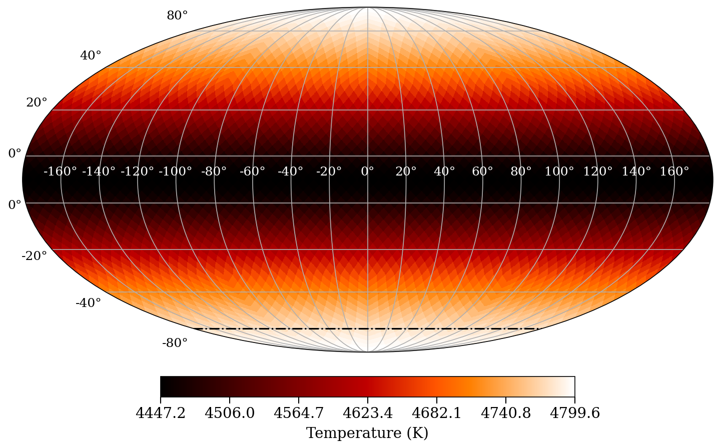
plot_mollweide(tmap, stars[1])

Data flow diagram

OIFITS files
    |
    v
readoifits_multiepochs()  -->  Vector{OIdata}  (one per epoch)
    |
    v
tessellation_healpix(n)   -->  tessellation     (unit sphere grid)
    |
    v
create_star_multiepochs() -->  Vector{stellar_geometry}
    |                           (rotated, projected, visibility-masked)
    v
setup_oi!()               -->  polyflux, polyft matrices stored in stars
    |
    v
image_reconstruct_oi()    -->  temperature map (Vector, length npix)
    |
    v
plot2d / plot_mollweide   -->  visualization

Example output

A Mollweide projection of the gravity-darkened temperature map for a rapid rotator: